Back in 2017, a bunch of Google researchers accidentally stumbled upon the AI equivalent of sliced bread. Their paper, modestly titled “Attention Is All You Need” (spoiler alert: it wasn’t), unleashed the Transformer architecture upon an unsuspecting world. Little did they know they’d just fired the starting pistol for a revolution in Natural Language Processing that would make the industrial revolution look like a minor software update. Fast forward to today, and Transformers have become the Swiss Army knife of NLP - the go-to solution for everything from completing your sentences to writing your college essays (not that I endorse that, of course ;). In this article, we’re going to dissect this AI superstar, peeking under the hood of the Transformer architecture. Buckle up, fellow geeks and AI enthusiasts - we’re about to transform your understanding of, well, Transformers. No Autobots or Decepticons were harmed in the making of this blog post.

What are Transformers, and why should you care?

No, we’re not talking about shape-shifting robots or those humming boxes outside your house. In the world of AI, Transformers are the cool kids on the block, the ones who showed up to the NLP party and refused to leave.

At their core, Transformers are a type of neural network architecture designed to handle sequential data, like text. But unlike their predecessors who insisted on processing data one element at a time (looking at you, RNNs), Transformers took one look at that idea and said, “Nah, let’s do it all at once.” Imagine you’re at a party (an AI party, of course), trying to understand a conversation. Old-school models would listen to each word one by one, struggling to remember what was said five minutes ago. Transformers, on the other hand, take in the whole conversation at once, paying attention to the important bits and casually ignoring your friend’s long-winded story about their cat.

The secret sauce? It’s called ‘self-attention’. This nifty mechanism allows Transformers to weigh the importance of different parts of the input when processing each part. It’s like having a super-smart friend at that AI party who can instantly connect what someone just said to something mentioned an hour ago. But here’s the kicker - Transformers don’t just excel at understanding language. They’ve crash-landed into other fields too, from generating images to composing music. They’re the overachievers of the AI world, making the rest of us feel a bit inadequate. In the following sections, we’ll dive deeper into how these show-offs actually work. We’ll even build our own mini-Transformer, because why should Google have all the fun? So grab your favorite caffeinated beverage, and let’s transform our understanding of Transformers!

The anatomy of a Transformer

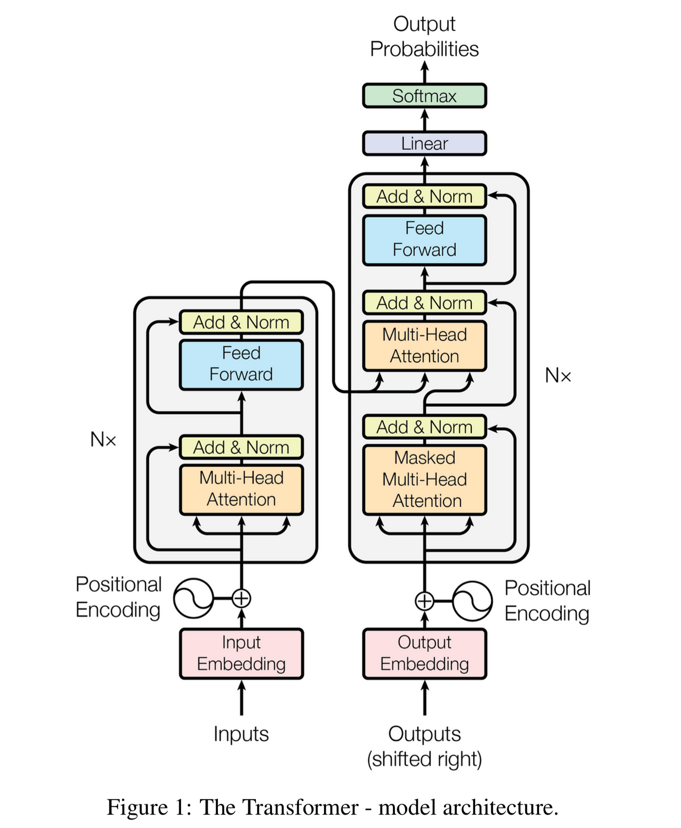
Picture a Transformer as a gourmet kitchen (stay with me here). You’ve got two main sections: the Encoder (let’s call it the prep station) and the Decoder (the cooking area). Between them, they’re going to turn your raw ingredients (input text) into a Michelin-star dish (output text).

The Encoder-Decoder Structure:

Our Transformer kitchen has a unique setup. The Encoder preps the ingredients, understanding and contextualizing the input. The Decoder then takes this prepped information and whips up the final dish. It’s like having a sous chef (Encoder) who perfectly understands your vision, working in tandem with the head chef (Decoder) to create culinary magic.

Key Components:

1. Self-Attention: This is our chef’s knife - the most crucial tool in the kitchen. It allows each word to look at other words in the input, figuring out how they relate to each other. It’s like each ingredient getting to know all the other ingredients intimately before the cooking begins.

2. Feed-Forward Networks: Think of these as the ovens. After the ingredients have mingled (self-attention), they each go through these ‘ovens’ for individual processing.

3. Layer Normalization: This is quality control. After each major step, we normalize the outputs, ensuring our dish maintains a consistent flavor throughout the cooking process.

Now, let’s get our hands dirty. We’re going to start building our own Transformer, piece by piece. Don’t worry if you’re not a coding Gordon Ramsay - we’ll take it step by step.

import torch
import torch.nn as nn
import math

class Transformer(nn.Module):
    def __init__(self, vocab_size, d_model, nhead, num_encoder_layers, num_decoder_layers):
        super(Transformer, self).__init__()
        # We'll fill this in as we go along
        pass

    def forward(self, src, tgt):
        # This too will be implemented step by step
        pass

# Don't worry about these parameters for now, we'll explain them later
model = Transformer(vocab_size=1000, d_model=512, nhead=8, num_encoder_layers=6, num_decoder_layers=6)

Let’s break this down:

We import torch and torch.nn. These are our main PyTorch ingredients, providing tensor computations and neural network layers.

We define a Transformer class that inherits from nn.Module, PyTorch’s base class for all neural network modules.

The init method takes several parameters:

vocab_size: The size of our vocabulary (how many unique words we’re working with)

d_model: The dimensionality of our model’s embeddings and hidden states

nhead: The number of attention heads (we’ll explain this later)

num_encoder_layers and num_decoder_layers: The number of encoder and decoder layers

The forward method is where the actual computation happens. We’ll implement this as we go along. Finally, we create an instance of our Transformer with some initial parameters

Input representation

Imagine trying to teach a computer to write like Shakespeare. First challenge: computers don’t speak English, let alone Elizabethan English. They prefer numbers - lots of them. So, how do we turn “To be, or not to be” into something a silicon brain can understand? Enter character-level encoding and embeddings - our digital quill and ink.

Character-level encoding: Every letter counts

Instead of breaking our text into words, we’re going to go even smaller - individual characters. It’s like taking Shakespeare’s works and putting each letter, space, and punctuation mark on its own tiny sticky note. This is not how OpenAI’s GPT-3 does it, but it’s a good starting point for our mini-Transformer.

Let’s use the first few lines from Hamlet in the Tiny Shakespeare dataset as our example:

text = """
First Citizen:
Before we proceed any further, hear me speak.

All:
Speak, speak.

First Citizen:
You are all resolved rather to die than to famish?
"""

class CharTokenizer:
    def __init__(self):
        self.chars = sorted(list(set(text)))
        self.char_to_idx = {ch: i for i, ch in enumerate(self.chars)}
        self.idx_to_char = {i: ch for i, ch in enumerate(self.chars)}
        self.vocab_size = len(self.chars)

    def encode(self, string):
        return [self.char_to_idx[ch] for ch in string]

    def decode(self, indices):
        return ''.join([self.idx_to_char[idx] for idx in indices])

tokenizer = CharTokenizer()
encoded = tokenizer.encode("To be, or not to be")
print(encoded)  # Output might be something like: [46, 15, 1, 2, 27, 7, 1, 15, 14, 1, 16, 15, 14, 1, 14, 15, 1, 2, 27]
print(tokenizer.decode(encoded))  # Output: "To be, or not to be"

This tokenizer creates a vocabulary from all unique characters in our text and converts each character to a unique index.

Embeddings: Giving Characters Meaning

Now that we’ve atomized our text into individual characters, we need to give each one some context. Enter embeddings - the Transformer’s way of understanding the essence of each character. Let’s add an embedding layer to our Transformer:

import torch
import torch.nn as nn

class Transformer(nn.Module):
    def __init__(self, vocab_size, d_model):
        super(Transformer, self).__init__()
        self.embedding = nn.Embedding(vocab_size, d_model)
        self.positional_encoding = PositionalEncoding(d_model)

    def forward(self, src):
        src = self.embedding(src)
        src = self.positional_encoding(src)
        return src

class PositionalEncoding(nn.Module):
    def __init__(self, d_model, max_len=5000):
        super(PositionalEncoding, self).__init__()
        # We'll implement this in the next section
        pass

    def forward(self, x):
        # We'll implement this in the next section
        return x

# Example usage
vocab_size = len(tokenizer.chars)
d_model = 512
model = Transformer(vocab_size, d_model)

input_sequence = torch.tensor(tokenizer.encode("To be, or not to be"))
output = model(input_sequence)
print(output.shape)  # Should print torch.Size([18, 512]) for our example

Here, nn.Embedding creates a lookup table that we’ll learn during training. Each character index gets mapped to a d_model-dimensional vector. In this case, we’re using a 512-dimensional embedding, but this can be adjusted based on the complexity of your task.

But why do we need embeddings?

You might be wondering, “We’ve already turned characters into numbers with our tokenizer. Why do we need to convert them again?” Great question! Let’s break it down:

1. One-Hot Encoding is Not Enough: If we just used the indices from our tokenizer, each character would be represented by a single number. This is essentially one-hot encoding, where ‘A’ might be [1,0,0,…], ‘B’ [0,1,0,…], and so on. While this uniquely identifies each character, it doesn’t capture any meaningful relationships between them.

2. Capturing Relationships: Embeddings allow our model to learn and represent complex relationships between characters. In the embedding space, characters that often appear in similar contexts (like ‘q’ and ‘u’ in English) might end up close to each other.

3. Dimensionality: Our vocabulary might only have 50-100 unique characters, but we’re embedding them into a much higher-dimensional space (512 dimensions in our example). This gives the model more ‘room’ to encode subtle differences and similarities.

4. Learned Representations: Unlike one-hot encoding, embeddings are learned during training. This means they can adapt to capture the most relevant features for our specific task and dataset.

5. Efficiency: Embeddings are much more computationally efficient than one-hot encodings, especially for subsequent layers in the network.

Here’s a simple analogy: Imagine you’re trying to describe colors to a colorblind friend. Instead of just giving each color a number (red is 1, blue is 2, etc.), you describe each color using multiple attributes like warmth, brightness, and association with objects. This richer description (embedding) allows your friend to understand the relationships between colors much better than just numbered labels.

Also, there’s a twist in our tale! Transformers, unlike humans, don’t read character by character. They look at the whole text at once, like a word search puzzle where all the letters are revealed. To help our model understand the order of characters, we add positional encoding. This is like numbering each of those tiny sticky notes before arranging them.

The Heart of Transformers : Attention Mechanism

Picture this: you’re at a party, and everyone’s chattering away. How do you focus on the most important conversations? That’s essentially what the attention mechanism does in Transformers. It helps the model focus on the most relevant parts of the input when processing information.

Self-attention is like having a conversation with yourself, but way cooler and more productive. It allows each word in a sequence to look at other words in the same sequence and figure out how important they are. Here’s how it works, step by step:

1. Query, Key, and Value Vectors

First, we create three vectors for each word: Query (Q), Key (K), and Value (V). Think of these as:

• Query: What you’re looking for
• Key: What you have to offer
• Value: The actual content you’re bringing to the table

Mathematically, we get these vectors by multiplying the input embedding (X) with weight matrices:

Q = XW_q
K = XW_k
V = XW_v

where W_q, W_k, and W_v are learnable weight matrices.

2. Calculating Attention Scores

Next, we calculate how much each word should attend to every other word. We do this by taking the dot product of the Query vector of one word with the Key vectors of all words:

Attention_scores = Q * K^T

3. Scale and apply softmax

To prevent the dot products from growing too large, we scale them by dividing by the square root of the dimension of the Key vectors (d_k). Then we apply the softmax function to get probabilities:

Attention_scores = Attention_scores / sqrt(d_k)
Attention_weights = softmax(Attention_scores)

4. Multiply with Values

Finally, we multiply the attention weights with the Value vectors to get the weighted sum:

Attention_output = Attention_weights * V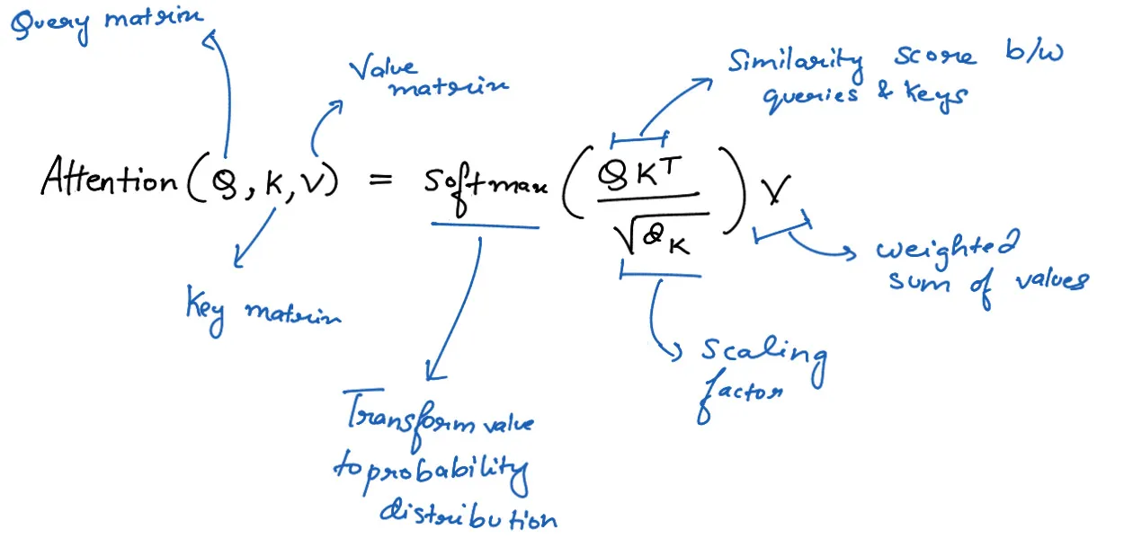

Now, let’s implement this all together in PyTorch:

class SelfAttention(nn.Module):
    def __init__(self, d_model, d_k):
        super(SelfAttention, self).__init__()
        self.W_Q = nn.Linear(d_model, d_k)
        self.W_K = nn.Linear(d_model, d_k)
        self.W_V = nn.Linear(d_model, d_k)

    def forward(self, X):
        Q = self.W_Q(X)
        K = self.W_K(X)
        V = self.W_V(X)

        attention_scores = torch.matmul(Q, K.transpose(-2, -1))
        attention_scores /= np.sqrt(K.size(-1))
        attention_weights = torch.nn.functional.softmax(attention_scores, dim=-1)
        output = torch.matmul(attention_weights, V)

        return output

This code implements the self-attention mechanism we just described. It takes an input X (a sequence of word embeddings) and returns an output where each word has “attended” to all other words in the sequence.

Remember, in the full Transformer architecture, this self-attention operation is typically repeated multiple times in parallel (multi-head attention) and is just one part of a larger structure including feed-forward networks, layer normalization, and residual connections.

Now, wasn’t that a party? We’ve just turned every word into a social butterfly, chatting with all the other words to figure out who’s most important. And that, my friends, is the magic of self-attention!

Multi-Head Attention: Because Two Heads (or More) Are Better Than One

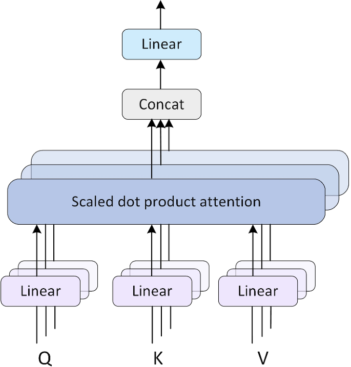
Now that we’ve mastered self-attention, let’s take it up a notch. Multi-head attention is like having multiple parallel universes of attention, each focusing on different aspects of the input. It’s the Transformer’s way of saying, “Why settle for one perspective when you can have many?”

Here’s how it works:

1. Create Multiple Sets of Q, K, V

Instead of having just one set of Query, Key, and Value matrices, we create multiple sets. Each set is called a “head”.

def create_attention_heads(X, num_heads, d_model, d_k):
    W_Q = [np.random.randn(d_model, d_k) for _ in range(num_heads)]
    W_K = [np.random.randn(d_model, d_k) for _ in range(num_heads)]
    W_V = [np.random.randn(d_model, d_k) for _ in range(num_heads)]

    Q = [np.dot(X, W_q) for W_q in W_Q]
    K = [np.dot(X, W_k) for W_k in W_K]
    V = [np.dot(X, W_v) for W_v in W_V]

    return Q, K, V

2. Apply Self-Attention in Parallel to Each Head

We perform the self-attention operation we learned earlier, but separately for each head.

def apply_attention(Q, K, V, d_k):
    attention_scores = np.dot(Q, K.T)
    attention_scores /= np.sqrt(d_k)
    attention_weights = np.exp(attention_scores) / np.sum(np.exp(attention_scores), axis=1, keepdims=True)
    return np.dot(attention_weights, V)

def multi_head_attention(Q, K, V, d_k):
    return [apply_attention(q, k, v, d_k) for q, k, v in zip(Q, K, V)]

3. Concatenate and Linear Transformation

After getting the outputs from each head, we concatenate them and apply a linear transformation to get the final multi-head attention output.

def combine_heads(attention_outputs, d_model):
    combined = np.concatenate(attention_outputs, axis=-1)
    W_O = np.random.randn(combined.shape[-1], d_model)
    return np.dot(combined, W_O)

Putting it all together, we get:

def multi_head_attention_layer(X, num_heads, d_model, d_k):
    Q, K, V = create_attention_heads(X, num_heads, d_model, d_k)
    attention_outputs = multi_head_attention(Q, K, V, d_k)
    return combine_heads(attention_outputs, d_model)

# Example usage
X = np.random.randn(5, 512)  # 5 words, each with 512-dimensional embedding
num_heads = 8
d_model = 512
d_k = d_model // num_heads

result = multi_head_attention_layer(X, num_heads, d_model, d_k)
print(result.shape)  # Should be (5, 512)

Why Multi-Head Attention?

Multi-head attention allows the model to jointly attend to information from different representation subspaces at different positions. In simple terms, it’s like having multiple experts look at the same problem from different angles:

1. One head might focus on syntactic relationships.
2. Another might capture semantic similarities.
3. A third could look at long-range dependencies.

By combining these diverse “viewpoints”, the model can capture richer and more nuanced relationships within the data.

The math behind multi-head attention

For those who love a good mathematical dive, here’s the multi-head attention formula in all its glory:

MultiHead(Q, K, V) = Concat(head_1, ..., head_h)WO
where head_i = Attention(QW_i^Q, KW_i^K, VW_i^V)

and the scaled dot-product attention function is:

Attention(Q, K, V) = softmax(QK^T / sqrt(d_k))V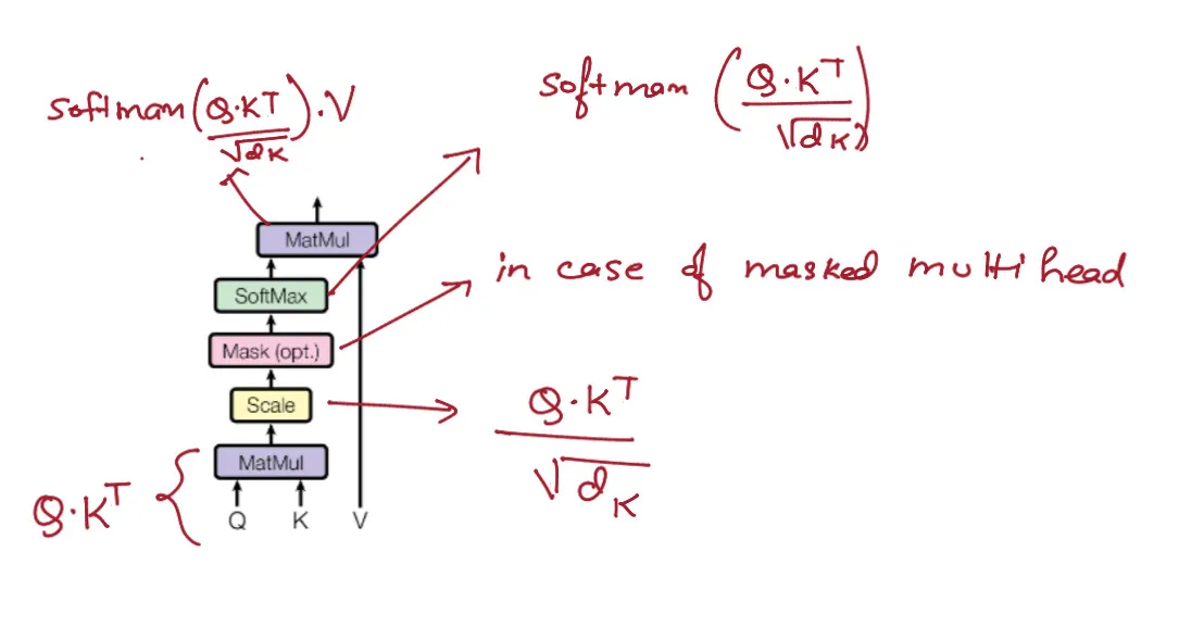

Transformer Encoder : The Prep Station

The Transformer Encoder is like the brain of our model - it takes in the input, processes it through multiple layers, and produces a rich, contextualized representation. Think of it as a high-tech assembly line for information processing.

Structure of the Encoder

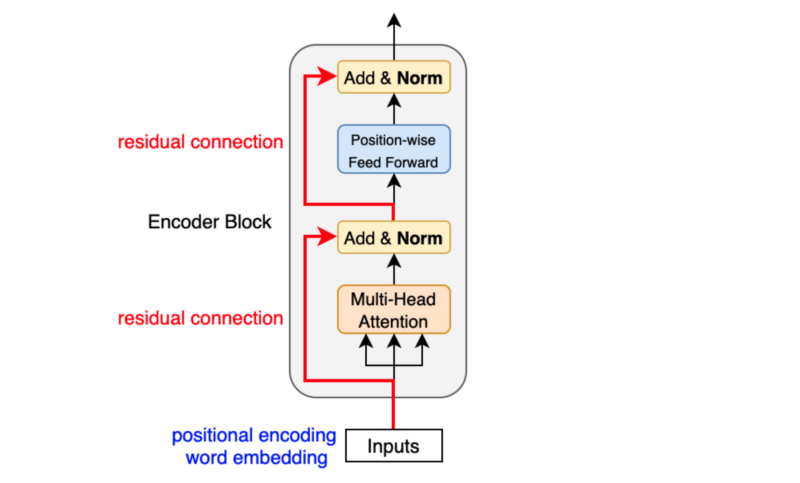
The Encoder consists of a stack of identical layers, each containing two main sub-layers:

1. Multi-Head Attention Layer
2. Position-wise Feed-Forward Networks

Each of these sub-layers is wrapped with a residual connection and followed by layer normalization. Let’s break it down:

1. Multi-Head Attention Layer We’ve already covered this in detail. The Encoder uses multi-head attention to capture different aspects of the input sequence in parallel. This allows the model to focus on different parts of the input and learn complex relationships between them.

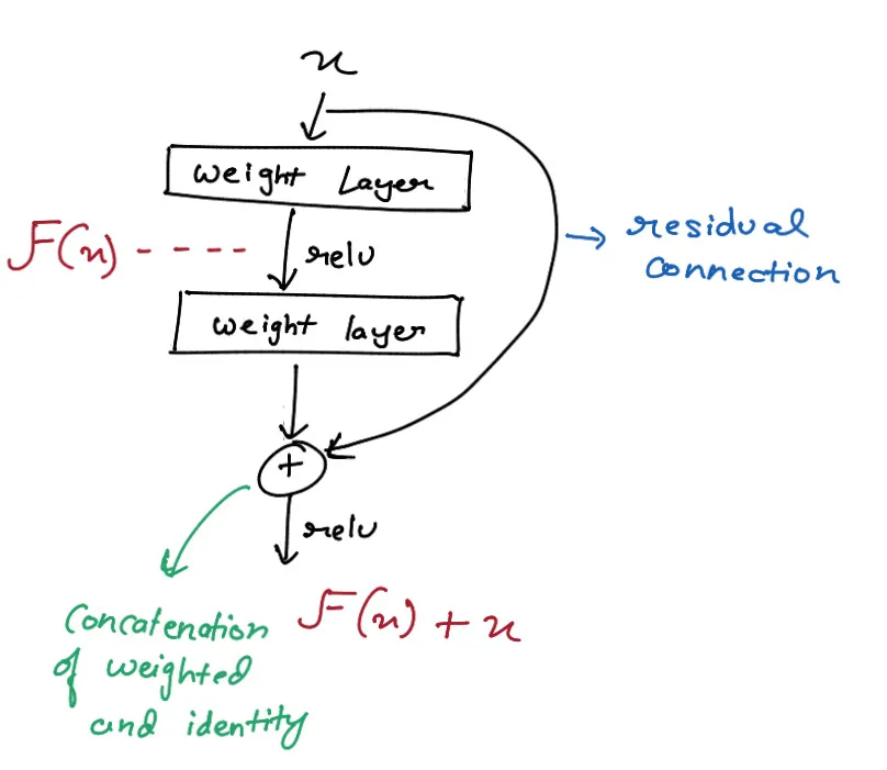
2. Position Wise Feed-Forward Networks This is a simple fully connected neural network applied to each position separately and identically. It typically consists of two linear transformations with a ReLU activation in between:

   FFN(x) = max(0, xW_1 + b_1)W_2 + b_2

3. Residual Connections These allow the model to bypass the sub-layers if needed, helping with training deep networks.

4. Layer Normalization This normalizes the output of each sub-layer before passing it to the next layer. It helps stabilize training and speeds up convergence.

Let’s implement everything we’ve learned so far into a full Transformer Encoder:

import torch
import torch.nn as nn
import torch.nn.functional as F

class MultiHeadAttention(nn.Module):
    def __init__(self, d_model, num_heads):
        super(MultiHeadAttention, self).__init__()
        self.num_heads = num_heads
        self.d_model = d_model

        assert d_model % self.num_heads == 0

        self.d_k = d_model // self.num_heads

        self.W_q = nn.Linear(d_model, d_model)
        self.W_k = nn.Linear(d_model, d_model)
        self.W_v = nn.Linear(d_model, d_model)
        self.W_o = nn.Linear(d_model, d_model)

    def scaled_dot_product_attention(self, Q, K, V, mask=None):
        attn_scores = torch.matmul(Q, K.transpose(-2, -1)) / torch.sqrt(torch.tensor(self.d_k, dtype=torch.float32))
        if mask is not None:
            attn_scores = attn_scores.masked_fill(mask == 0, -1e9)
        attn_probs = F.softmax(attn_scores, dim=-1)
        output = torch.matmul(attn_probs, V)
        return output

    def forward(self, x, mask=None):
        batch_size = x.size(0)

        Q = self.W_q(x)
        K = self.W_k(x)
        V = self.W_v(x)

        Q = Q.view(batch_size, -1, self.num_heads, self.d_k).transpose(1, 2)
        K = K.view(batch_size, -1, self.num_heads, self.d_k).transpose(1, 2)
        V = V.view(batch_size, -1, self.num_heads, self.d_k).transpose(1, 2)

        output = self.scaled_dot_product_attention(Q, K, V, mask)

        output = output.transpose(1, 2).contiguous().view(batch_size, -1, self.d_model)

        return self.W_o(output)

class PositionWiseFeedForward(nn.Module):
    def __init__(self, d_model, d_ff):
        super(PositionWiseFeedForward, self).__init__()
        self.fc1 = nn.Linear(d_model, d_ff)
        self.fc2 = nn.Linear(d_ff, d_model)

    def forward(self, x):
        return self.fc2(F.relu(self.fc1(x)))

class EncoderLayer(nn.Module):
    def __init__(self, d_model, num_heads, d_ff, dropout=0.1):
        super(EncoderLayer, self).__init__()
        self.self_attn = MultiHeadAttention(d_model, num_heads)
        self.feed_forward = PositionWiseFeedForward(d_model, d_ff)
        self.norm1 = nn.LayerNorm(d_model)
        self.norm2 = nn.LayerNorm(d_model)
        self.dropout = nn.Dropout(dropout)

    def forward(self, x, mask=None):
        attn_output = self.self_attn(x, mask)
        x = self.norm1(x + self.dropout(attn_output))
        ff_output = self.feed_forward(x)
        x = self.norm2(x + self.dropout(ff_output))
        return x

class TransformerEncoder(nn.Module):
    def __init__(self, num_layers, d_model, num_heads, d_ff, dropout=0.1):
        super(TransformerEncoder, self).__init__()
        self.layers = nn.ModuleList([EncoderLayer(d_model, num_heads, d_ff, dropout) for _ in range(num_layers)])

    def forward(self, x, mask=None):
        for layer in self.layers:
            x = layer(x, mask)
        return x

# Example usage
sequence_length = 5
batch_size = 2
d_model = 512
num_layers = 6
num_heads = 8
d_ff = 2048

x = torch.randn(batch_size, sequence_length, d_model)
encoder = TransformerEncoder(num_layers, d_model, num_heads, d_ff)
encoded = encoder(x)
print(encoded.shape)  # Should be (2, 5, 512)

This code implements a full Transformer Encoder. Let’s break down what’s happening:

1. We define helper functions for layer normalization and the feed-forward network.
2. The encoder_layer function implements a single layer of the encoder, including multi-head attention, feed-forward network, residual connections, and layer normalization.
3. The transformer_encoder function stacks multiple encoder layers.

Each time the input passes through an encoder layer, it gets a richer representation of the sequence. It’s like the input is going through multiple rounds of sophisticated analysis, each time gaining a deeper understanding of the context and relationships within the data.

The magic of the Transformer Encoder lies in its ability to process all positions of the input sequence in parallel, unlike recurrent neural networks which process sequentially. This parallelization is what makes Transformers so efficient and powerful. Remember, in the context of a language model like GPT, we’re using only the encoder part of the original Transformer architecture. The encoded representations produced by this encoder will be used directly by the subsequent layers to generate text.

By stacking multiple encoder layers, we’re giving our model the ability to learn increasingly abstract and complex representations of the input data. It’s like giving our AI multiple passes to really understand the nuances of the text it’s processing.

Transformer Decoder : The Cooking Area

The decoder is responsible for generating output sequences, making it the core of text generation in many language models.

Structure and Components

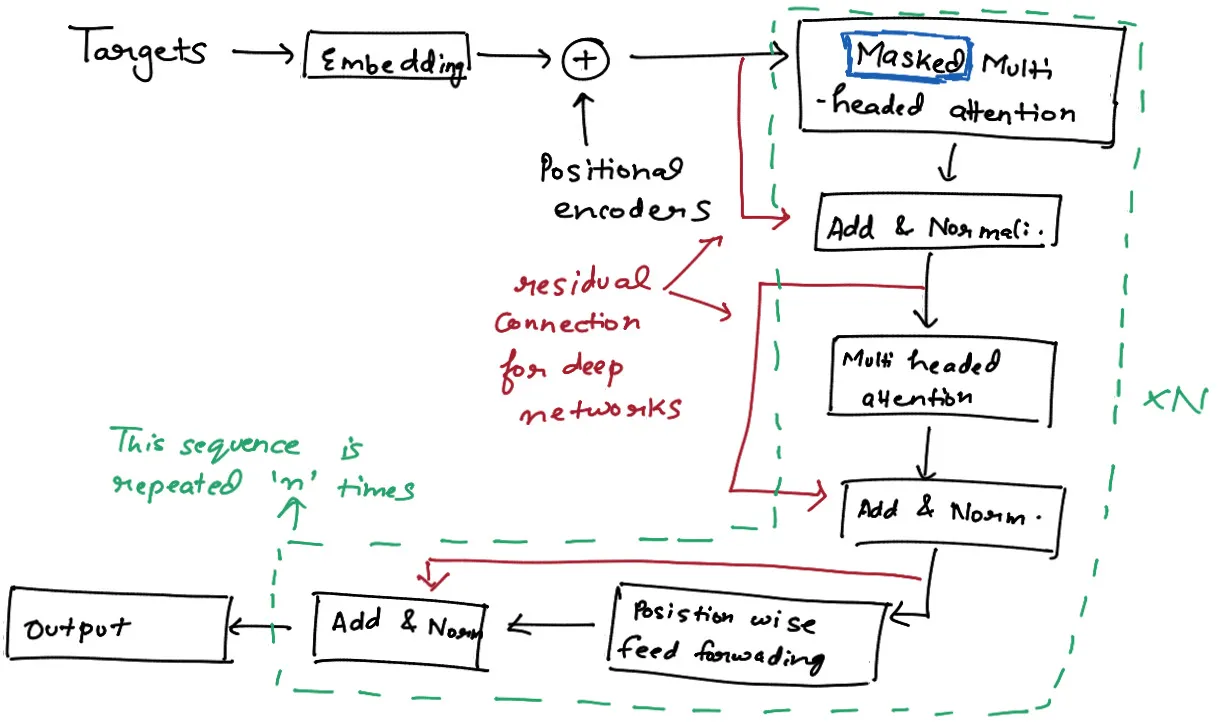
The Transformer Decoder is similar to the Encoder but with some key differences:

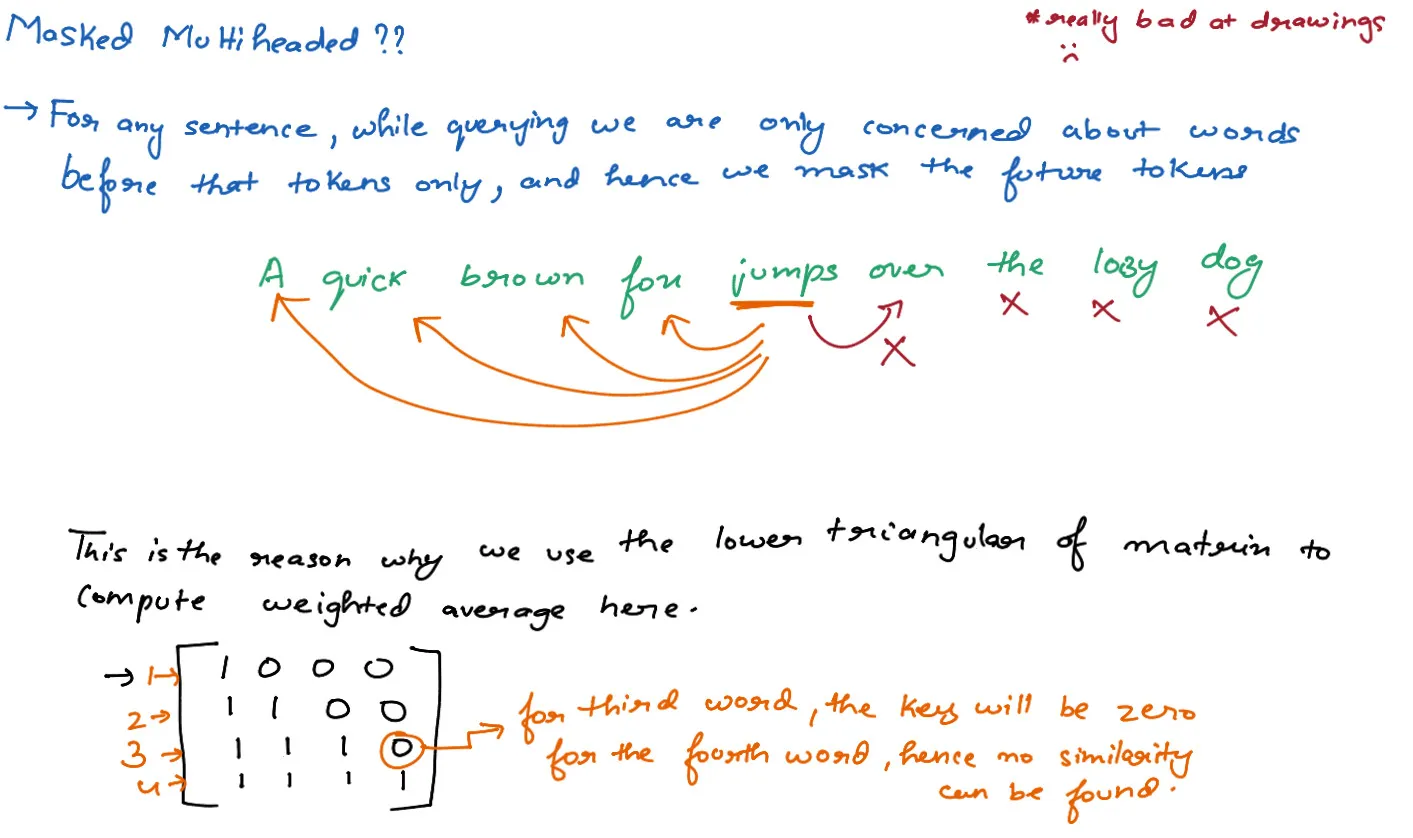
1. It has an additional attention layer that attends to the output of the encoder (masked multi-head attention)
2. The self-attention layer in the decoder is modified to prevent positions from attending to subsequent positions. This is done by masking future positions.

The main components of each decoder layer are:

• Masked Multi-Head Attention
• Multi-Head Attention (attending to encoder output)
• Position-wise Feed-Forward Network
• Layer Normalization and Residual Connections

Let’s implement the Transformer Decoder in PyTorch:

class DecoderLayer(nn.Module):
    def __init__(self, d_model, num_heads, d_ff, dropout=0.1):
        super(DecoderLayer, self).__init__()
        self.self_attn = MultiHeadAttention(d_model, num_heads)
        self.src_attn = MultiHeadAttention(d_model, num_heads)
        self.feed_forward = PositionWiseFeedForward(d_model, d_ff)
        self.norm1 = nn.LayerNorm(d_model)
        self.norm2 = nn.LayerNorm(d_model)
        self.norm3 = nn.LayerNorm(d_model)
        self.dropout = nn.Dropout(dropout)

    def forward(self, x, encoder_output, src_mask=None, tgt_mask=None):
        self_attn_output = self.self_attn(x, tgt_mask)
        x = self.norm1(x + self.dropout(self_attn_output))

        src_attn_output = self.src_attn(x, encoder_output, src_mask)
        x = self.norm2(x + self.dropout(src_attn_output))

        ff_output = self.feed_forward(x)
        x = self.norm3(x + self.dropout(ff_output))

        return x

class TransformerDecoder(nn.Module):
    def __init__(self, num_layers, d_model, num_heads, d_ff, dropout=0.1):
        super(TransformerDecoder, self).__init__()
        self.layers = nn.ModuleList([DecoderLayer(d_model, num_heads, d_ff, dropout) for _ in range(num_layers)])

    def forward(self, x, encoder_output, src_mask=None, tgt_mask=None):
        for layer in self.layers:
            x = layer(x, encoder_output, src_mask, tgt_mask)
        return x

Key points about this implementation:

1. The DecoderLayer includes both self-attention and cross-attention mechanisms. The self-attention allows the decoder to consider previous outputs, while the cross-attention allows it to focus on relevant parts of the input sequence.
2. We use masking in the self-attention layer (tgt_mask) to prevent positions from attending to subsequent positions. This is crucial for maintaining the auto-regressive property during generation.
3. The src_mask is used in the cross-attention layer to potentially mask out padding tokens in the source sequence.
4. The decoder takes both the previous output (x) and the encoder output (enc_output) as inputs.

In a GPT model, which is a decoder-only transformer, you would typically:

• Use only the self-attention mechanism (removing the cross-attention).
• Apply causal masking to ensure that predictions for a given token can depend only on the known outputs at earlier positions.

Positional Encoding : The Secret Sauce

We haven’t yet talked about how Transformers handle the sequential nature of text data. After all, words in a sentence have a specific order that carries meaning. This is where positional encoding comes in.

In sequence models like RNNs, the order of inputs is implicitly handled by the sequential nature of the processing. However, Transformers process all inputs in parallel, which means they need an explicit way to understand the position of each token in the sequence. This is where Positional Encoding comes in.

Key points about Positional Encoding:

1. Added to the input embeddings to provide information about the position of tokens.
2. Provides a way for the model to differentiate between tokens based on their position in the sequence.
3. Should be unique for each position, allowing the model to learn positional relationships.
4. Should have consistent patterns that the model can learn from.

The standard positional encoding used in the original Transformer model is based on sine and cosine functions of different frequencies. This allows the model to learn positional relationships based on the angle and position in the sequence.

PE(pos, 2i) = sin(pos / 10000^(2i/d_model))
PE(pos, 2i+1) = cos(pos / 10000^(2i/d_model))
where pos is the position and i is the dimension of the embedding

Let’s implement positional encoding in PyTorch:

import torch
import torch.nn as nn
import math

class PositionalEncoding(nn.Module):
    def __init__(self, d_model, max_len=5000):
        super(PositionalEncoding, self).__init__()

        # Create a long enough 'P'
        pe = torch.zeros(max_len, d_model)
        position = torch.arange(0, max_len, dtype=torch.float).unsqueeze(1)
        div_term = torch.exp(torch.arange(0, d_model, 2).float() * (-math.log(10000.0) / d_model))

        pe[:, 0::2] = torch.sin(position * div_term)
        pe[:, 1::2] = torch.cos(position * div_term)

        pe = pe.unsqueeze(0).transpose(0, 1)

        # Register buffer (not a parameter of the model)
        self.register_buffer('pe', pe)

    def forward(self, x):
        return x + self.pe[:x.size(0), :]

# Example usage
d_model = 512
max_len = 100
batch_size = 32
seq_len = 20

pos_encoder = PositionalEncoding(d_model, max_len)

# Simulate input embeddings
x = torch.randn(seq_len, batch_size, d_model)

encoded = pos_encoder(x)
print(encoded.shape)  # Should be (20, 32, 512)

Let’s break down what’s happening here:

1. We create a matrix pe of size (max_len, d_model) to store the positional encodings.
2. We use broadcasting to compute the sine and cosine values for all positions and dimensions at once:
   • position * div_term creates a matrix where each row corresponds to a position and each column to a frequency.
   • We then apply sin to even indices and cos to odd indices.
3. In the forward pass, we simply add the appropriate slice of this encoding to our input.

The resulting encoding has several useful properties:

• It’s deterministic, so the model always sees the same encoding for the same position.
• It can extrapolate to sequences longer than it has seen during training.
• The sine and cosine functions at different frequencies allow the model to easily attend to relative positions. For any fixed offset k, PE(pos+k) can be represented as a linear function of PE(pos).

Output Layer : Bringing It All Together

The output layer is responsible for transforming the high-dimensional representations produced by the Transformer layers into predictions. In the case of a language model, these predictions are typically probabilities over the vocabulary for the next token in the sequence.

Key Components:

1. Final Linear Layer
2. Softmax Activation

Let’s implement this in PyTorch:

import torch
import torch.nn as nn
import torch.nn.functional as F

class TransformerOutputLayer(nn.Module):
    def __init__(self, d_model, vocab_size):
        super(TransformerOutputLayer, self).__init__()
        self.linear = nn.Linear(d_model, vocab_size)

    def forward(self, x):
        # x shape: (batch_size, seq_len, d_model)
        logits = self.linear(x)
        # logits shape: (batch_size, seq_len, vocab_size)
        return logits

class GPTModel(nn.Module):
    def __init__(self, vocab_size, d_model, nhead, num_layers, d_ff, max_seq_length, dropout=0.1):
        super(GPTModel, self).__init__()
        self.d_model = d_model

        self.embedding = nn.Embedding(vocab_size, d_model)
        self.positional_encoding = PositionalEncoding(d_model, max_seq_length)

        decoder_layers = nn.TransformerDecoderLayer(d_model, nhead, d_ff, dropout)
        self.transformer_decoder = nn.TransformerDecoder(decoder_layers, num_layers)

        self.output_layer = TransformerOutputLayer(d_model, vocab_size)

    def forward(self, src, src_mask=None):
        # src shape: (batch_size, seq_len)

        # Embedding + Positional Encoding
        src = self.embedding(src) * math.sqrt(self.d_model)
        src = self.positional_encoding(src)

        # Transformer Decoder (used as a decoder-only model)
        output = self.transformer_decoder(src, src, tgt_mask=src_mask)

        # Output layer
        logits = self.output_layer(output)

        return logits

    def generate(self, input_ids, max_length):
        self.eval()
        with torch.no_grad():
            for _ in range(max_length - len(input_ids)):
                # Prepare input
                input_tensor = torch.tensor(input_ids).unsqueeze(0)  # Add batch dimension

                # Create mask
                src_mask = (torch.triu(torch.ones(len(input_ids), len(input_ids))) == 1).transpose(0, 1)
                src_mask = src_mask.float().masked_fill(src_mask == 0, float('-inf')).masked_fill(src_mask == 1, float(0.0))

                # Forward pass
                logits = self(input_tensor, src_mask)

                # Get the next token prediction
                next_token_logits = logits[0, -1, :]
                next_token = torch.argmax(next_token_logits).item()

                # Append to input_ids
                input_ids.append(next_token)

                # Stop if we predict the end of sequence token
                if next_token == your_eos_token_id:
                    break

        return input_ids

# Example usage
vocab_size = 10000
d_model = 512
nhead = 8
num_layers = 6
d_ff = 2048
max_seq_length = 1024
batch_size = 32
seq_len = 20

model = GPTModel(vocab_size, d_model, nhead, num_layers, d_ff, max_seq_length)

# Simulate input tokens
src = torch.randint(0, vocab_size, (batch_size, seq_len))

# Create a triangular mask to ensure causality
src_mask = (torch.triu(torch.ones(seq_len, seq_len)) == 1).transpose(0, 1)
src_mask = src_mask.float().masked_fill(src_mask == 0, float('-inf')).masked_fill(src_mask == 1, float(0.0))

logits = model(src, src_mask)
print(logits.shape)  # Should be (32, 20, 10000)

# Generate some text
input_ids = [234, 345, 456]  # Some initial tokens
your_eos_token_id = 1  # Assuming 1 is your end-of-sequence token
generated = model.generate(input_ids, max_length=50)
print(generated)

Let’s break down the key components:

1. TransformerOutputLayer
   • This layer takes the high-dimensional output from the Transformer (shape: batch_size x seq_len x d_model) and projects it to the vocabulary size.
   • The output (logits) has shape: batch_size x seq_len x vocab_size.
2. GPTModel
   • This is a complete GPT-style model, using the Transformer decoder as a decoder-only model.
   • It includes embedding, positional encoding, Transformer layers, and the output layer.
   • The forward method processes input sequences and returns logits.
   • The generate method demonstrates how to use the model for text generation.
3. Output Processing
   • In the forward method, we simply return the logits.
   • For training, you would typically pass these logits to a loss function along with the true next tokens.
   • For inference (as in the generate method), we use torch.argmax to select the most likely next token.
4. Text Generation
   • The generate method shows how to use the model to generate text autoregressively.
   • It uses a triangular mask to ensure the model only attends to previous tokens when predicting the next one.
   • It generates tokens one by one until reaching the maximum length or predicting an end-of-sequence token.

This output layer, combined with the rest of the Transformer architecture, allows the model to learn to predict the next token in a sequence based on all previous tokens, enabling it to generate coherent and contextually relevant text.

Conclusion

We’ve journeyed through the intricate architecture of Transformer models, specifically focusing on the GPT (Generative Pre-trained Transformer) style. Let’s recap what we’ve learned and discuss the implications:

1. Architecture Overview We explored the key components of Transformers, including:

   • Multi-Head Attention
   • Positional Encoding
   • Feed-Forward Networks
   • Layer Normalization and Residual Connections
   • The Encoder-Decoder Structure - The Output Layer

2. The Power of Self-Attention We saw how self-attention allows the model to weigh the importance of different parts of the input sequence dynamically. This is a game-changer for processing sequential data, enabling the model to capture long-range dependencies more effectively than traditional RNNs.

3. Scalability and Parallelization Unlike recurrent models, Transformers process entire sequences in parallel, making them highly efficient on modern hardware. This allows for training on massive datasets, which is crucial for their impressive performance.

4. Versatility While we focused on language modeling, the Transformer architecture has proven effective across a wide range of tasks, from machine translation to image generation.

5. Challenges and Future Directions Transformers have revolutionized the field of natural language processing, but they’re not without challenges. Training large models requires significant computational resources, and fine-tuning for specific tasks can be data-intensive. Researchers are exploring ways to make Transformers more efficient and adaptable to different domains.

Building your own GPT

By implementing each component of the Transformer architecture, we’ve demystified these powerful models. While our implementation is a simplified version, it captures the core principles that drive state-of-the-art language models.

Remember, the true power of models like GPT comes not just from their architecture, but from the vast amounts of data they’re trained on and the computational resources used. However, understanding the fundamentals as we’ve done here is crucial for anyone looking to work with or improve upon these models.

As you continue your journey in the world of natural language processing and deep learning, keep experimenting, stay curious, and always consider the ethical implications of the technology you’re working with.

The field of AI and language models is rapidly evolving, and who knows? The next breakthrough could come from someone like you, armed with the knowledge we’ve explored in this blog post.

Happy coding, and may your models generate wisely!

The Entire Code in One Place

Google Colab Link

import torch
import torch.nn as nn
from torch.nn import functional as F

# Hyperparameters
batch_size = 16          # Number of independent sequences to run in parallel
block_size = 32          # Maximum context length for predictions
max_iters = 5000         # Maximum number of iterations to train the model
eval_interval = 100      # Interval at which to evaluate the model
learning_rate = 1e-3     # Learning rate for the optimizer
device = torch.device("cuda" if torch.cuda.is_available() else "cpu")  # Using GPU if available
eval_iters = 200         # Number of iterations to run evaluation for
n_embd = 64              # Number of dimensions in the embedding
n_head = 4               # Number of heads in the multi-head attention
n_layer = 4              # Number of layers in the transformer
dropout = 0.1            # Dropout rate to prevent overfitting
torch.manual_seed(0)     # Setting the random seed for reproducibility

# Importing tiny Shakespeare dataset
with open('input.txt', 'r') as f:
    text = f.read()

# Unique characters in the text
chars = sorted(list(set(text)))
vocab_size = len(chars)  # Number of unique characters in the text

# Create dictionaries for character to index (stoi) and index to character (itos) mappings
stoi = { ch: i for i, ch in enumerate(chars) }
itos = { i: ch for i, ch in enumerate(chars) }

# Function to encode text into a list of indices
def encode(text):
    return torch.tensor([stoi[ch] for ch in text], dtype=torch.long)

# Function to decode a list of indices into text
def decode(tensor):
    return ''.join([itos[i] for i in tensor])

# Encode the entire dataset
data = encode(text)
n = int(len(data) * 0.8)  # 80% train, 20% test
train_data = data[:n]     # Training data
val_data = data[n:]       # Validation data

# Function to get a batch of data
def get_batch(split):
    data = train_data if split == 'train' else val_data
    ix = torch.randint(len(data) - block_size, (batch_size,))
    x = torch.stack([data[i:i+block_size] for i in ix])
    y = torch.stack([data[i+1:i+block_size+1] for i in ix])
    x, y = x.to(device), y.to(device)  # Move to GPU if available
    return x, y

# One head of the self-attention mechanism
class Head(nn.Module):
    def __init__(self, head_size):
        super().__init__()
        self.key = nn.Linear(n_embd, head_size, bias=False)
        self.query = nn.Linear(n_embd, head_size, bias=False)
        self.value = nn.Linear(n_embd, head_size, bias=False)
        self.register_buffer('tril', torch.tril(torch.ones(block_size, block_size)))
        self.dropout = nn.Dropout(dropout)

    def forward(self, x):
        B, T, C = x.shape
        k = self.key(x)
        q = self.query(x)
        wei = q @ k.transpose(-2, -1) / (C ** 0.5)
        wei = wei.masked_fill(self.tril[:T, :T] == 0, float('-inf'))
        wei = F.softmax(wei, dim=-1)
        wei = self.dropout(wei)
        v = self.value(x)
        out = wei @ v
        return out

# Multi-head attention mechanism
class MultiHeadAttention(nn.Module):
    def __init__(self, num_heads, head_size):
        super().__init__()
        self.heads = nn.ModuleList([Head(head_size) for _ in range(num_heads)])
        self.proj = nn.Linear(n_embd, n_embd)
        self.dropout = nn.Dropout(dropout)

    def forward(self, x):
        out = torch.cat([h(x) for h in self.heads], dim=-1)
        out = self.dropout(self.proj(out))
        return out

# Feedforward network with one hidden layer
class FeedForward(nn.Module):
    def __init__(self, n_embd):
        super().__init__()
        self.net = nn.Sequential(
            nn.Linear(n_embd, 4*n_embd),
            nn.ReLU(),
            nn.Linear(4*n_embd, n_embd),
            nn.Dropout(dropout)
        )

    def forward(self, x):
        return self.net(x)

# Transformer block: Multi-head attention followed by feedforward network
class Block(nn.Module):
    def __init__(self):
        super().__init__()
        head_size = n_embd // n_head
        self.sa = MultiHeadAttention(n_head, head_size)
        self.ffwd = FeedForward(n_embd)
        self.ln1 = nn.LayerNorm(n_embd)
        self.ln2 = nn.LayerNorm(n_embd)

    def forward(self, x):
        x = x + self.sa(self.ln1(x))
        x = x + self.ffwd(self.ln2(x))
        return x

# GPT model
class GPT(nn.Module):
    def __init__(self):
        super().__init__()
        self.emb = nn.Embedding(vocab_size, n_embd)
        self.position_embedding_table = nn.Embedding(block_size, n_embd)
        self.blocks = nn.Sequential(*[Block() for _ in range(n_layer)])
        self.ln = nn.LayerNorm(n_embd)
        self.lm_head = nn.Linear(n_embd, vocab_size)

    def forward(self, idx, targets=None):
        B, T = idx.shape
        tok_emb = self.emb(idx)
        pos_emb = self.position_embedding_table(torch.arange(T, device=device))
        x = tok_emb + pos_emb
        x = self.blocks(x)
        x = self.ln(x)
        logits = self.lm_head(x)

        if targets is None:
            loss = None
        else:
            B, T, C = logits.shape
            logits = logits.view(B * T, C)
            targets = targets.view(B * T)
            loss = F.cross_entropy(logits, targets)

        return logits, loss

    def generate(self, idx, max_new_tokens):
        for _ in range(max_new_tokens):
            idx_cond = idx if idx.size(1) <= block_size else idx[:, -block_size:]
            logits, _ = self(idx_cond)
            logits = logits[:, -1, :]
            probs = F.softmax(logits, dim=-1)
            idx_next = torch.multinomial(probs, num_samples=1)
            idx = torch.cat([idx, idx_next], dim=-1)
        return idx

@torch.no_grad()
def estimate_loss(model):
    out = {}
    model.eval()
    for split in ['train', 'val']:
        losses = torch.zeros(eval_iters, device=device)
        for k in range(eval_iters):
            x, y = get_batch(split)
            _, loss = model(x, y)
            losses[k] = loss.item()
        out[split] = losses.mean().item()
    model.train()
    return out

model = GPT().to(device)
print(sum(p.numel() for p in model.parameters() if p.requires_grad))

optimizer = torch.optim.Adam(model.parameters(), lr=learning_rate)

for iter in range(max_iters):
    if iter % eval_interval == 0:
        losses = estimate_loss(model)
        print(f"iter {iter} train loss: {losses['train']} val loss: {losses['val']}")

    x, y = get_batch('train')
    logits, loss = model(x, y)
    optimizer.zero_grad()
    loss.backward()
    optimizer.step()

context = torch.zeros((1, 1), dtype=torch.long, device=device)
generated_text = model.generate(context, 1000)
print(decode(generated_text[0].tolist()))

Resources and References

This blog post was inspired by the incredible work of researchers and educators in the field of deep learning. Here are some resources used while creating this content:

1. Attention Is All You Need (Original Transformer Paper)
2. The Illustrated Transformer (Excellent Blog by Jalammar)
3. Attention in transformers, visually explained by 3blue1brown
4. Illustrated Guide to Transformers Neural Network (If you are more of a visual guy)
5. Let’s build GPT: from scratch, in code, spelled out by Andrej Karpathy

Research paper you might want to read

Learning is a never ending process, here are some research papers you might want to read to dive deep into the world of transformers.

1. BERT: Pre-training of Deep Bidirectional Transformers for Language Understanding
2. GPT-3: Language Models are Few-Shot Learners
3. Dropout : A Simple Way to Prevent Neural Networks from Overfitting
4. Long Short-Term Memory
5. LoRA : Low Rank Adaptation of Large Language Models